Introduction to NLTK (Natural Language Processing) with Python

0. Introduction to NLP and Sentiment Analysis
1. Natural Language Processing with NTLK
3. Build a sentiment analysis program
4. Sentiment Analysis with Twitter
5. Analysing the Enron Email Corpus
6. Build a Spam Filter using the Enron Corpus
This first video is just a quick introduction to the NTLK library in Python.
All the source code for this and the upcoming videos is here.
You need to download some data sources before. Run these commands (instructions in video as well):
import nltk
nltk.download()
Be prepared for it to take some time. There is one file I mention in the video- panlex_lite or something. Don’t download that, or just press cancel when it is downloading that file (because it is huge, and pretty useless).
Everything else should be easy.
Only interested in the video? Go to part 2 here: Intro to NTLK, Part 2
There is a great completely free book for learning Natural Language Processing at http://www.nltk.org/book/
It also introduces you to Python if you are new to it. But there is a lot of information there, and it an be a bit overwhelming. What we will try to do in this lesson is, go over the main features of the Python NLTK library.
import nltk.classify.util
from nltk.classify import NaiveBayesClassifier
from nltk.corpus import movie_reviews
from nltk.corpus import stopwords
from nltk.tokenize import word_tokenize
from nltk.corpus import wordnet
We import everything we need. We will go over these functions as we use them.
To start off, say we have a sentence, and we want to extract all the words from it.
sentence = "The Quick brown fox, Jumps over the lazy little dog. Hello World."
sentence.split(" ")

['The',
 'Quick',
 'brown',
 'fox,',
 'Jumps',
 'over',
 'the',
 'lazy',
 'little',
 'dog.',
 'Hello',
 'World.']
We can split the function on a space (” “) to get all the words. The problem with this is, we cannot extract punctuation marks like full stops, and this simple parser will not be able to handle every single type of sentence.
Which is why we should use the word tokenizer provided by the NLTK library. This correctly identifies punctuation marks:
word_tokenize(sentence)

['The',
 'Quick',
 'brown',
 'fox',
 ',',
 'Jumps',
 'over',
 'the',
 'lazy',
 'little',
 'dog',
 '.',
 'Hello',
 'World',
 '.']
The word_tokenize() function is very useful, and we will be using it later.
Another useful feature is that nltk can figure out if a parts of a sentence are nouns, adverbs, verbs etc.
The pos_tag() works on the output of word_tokenize():
w = word_tokenize(sentence)
nltk.pos_tag(w)

[('The', 'DT'),
 ('Quick', 'NNP'),
 ('brown', 'NN'),
 ('fox', 'NN'),
 (',', ','),
 ('Jumps', 'NNP'),
 ('over', 'IN'),
 ('the', 'DT'),
 ('lazy', 'JJ'),
 ('little', 'JJ'),
 ('dog', 'NN'),
 ('.', '.'),
 ('Hello', 'NNP'),
 ('World', 'NNP'),
 ('.', '.')]
If you want to know what those tags mean, you can search for them online, or use the inbuilt functions:
nltk.help.upenn_tagset()
So for example, NN means singular noun, JJ means adjective etc.
The Nltk has many great features, like finding the meaning of words, finding examples of words, finding similar and opposite words etc. You can see how useful these features would be if you were building like a search engine, or a text parser.
Let’s look at a few of these features.
The first thing you can do it, find the definition of any word.
syn = wordnet.synsets("computer")
print(syn)
print(syn[0].name())
print(syn[0].definition())

print(syn[1].name())
print(syn[1].definition())

[Synset('computer.n.01'), Synset('calculator.n.01')]
computer.n.01
a machine for performing calculations automatically
calculator.n.01
an expert at calculation (or at operating calculating machines)
The name() function gives the internal name of the word, since a word can have multiple definitions. In the example above, the word computer can mean the machine (stored internally as computer.n.01), or a human who performs calculations (stored as calculator.n.01).
Interesting side history in no way related to this lesson: until World War II, computers were humans, usually women, whose job was to manually calculate the trajectories of missiles, artillery etc. Of course, they had cheat sheets, but they did the calculations by hand. Only after WWII, when computers became fast enough to do this job, did the word computer come to mean the machine. The definition above makes the distinction between the words.
You can also look at example usage of words:
syn = wordnet.synsets("talk")
syn[0].examples()

["let's have more work and less talk around here"]
Very useful advice- for me!
If you don’t know what hyponyms and hypernyms are, the Wikipedia page is a good place to look. Actually, just the main image gives you a good idea:
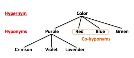
Hypernym is the root of the word, color in the image above. Hyponyms are similar words, like the colors red blue green etc.
syn = wordnet.synsets("speak")[0]

print(syn.hypernyms())

print(syn.hyponyms())

[Synset('communicate.v.02')]

[Synset('babble.v.01'), Synset('bark.v.01'), Synset('bay.v.01'), Synset('begin.v.04'),
Synset('blubber.v.02'), Synset('blurt_out.v.01'), Synset('bumble.v.03'),
Synset('cackle.v.01'), Synset('chatter.v.04'), Synset('chatter.v.05'),
Synset('deliver.v.01'), Synset('drone.v.02'), Synset('enthuse.v.02'),
Synset('generalize.v.02'), Synset('gulp.v.02'), Synset('hiss.v.03'),
Synset('lip_off.v.01'), Synset('mumble.v.01'), Synset('murmur.v.01'),
Synset('open_up.v.07'), Synset('peep.v.04'), Synset('rant.v.01'),
Synset('rasp.v.02'), Synset('read.v.03'), Synset('shout.v.01'), Synset('sing.v.02'),
Synset('slur.v.03'), Synset('snap.v.01'), Synset('snivel.v.01'), Synset('speak_in_tongues.v.01'),
Synset('speak_up.v.02'), Synset('swallow.v.04'), Synset('talk_of.v.01'),
Synset('tone.v.01'), Synset('tone.v.02'), Synset('troll.v.07'), Synset('verbalize.v.01'),
Synset('vocalize.v.05'), Synset('whiff.v.05'), Synset('whisper.v.01'), Synset('yack.v.01')]
You can see communicate is the root (hypernym) of speak, while there are dozens of similar words. Babble, chatter, rant, troll, yack are a few.
What if you want to find the opposite word (antonym) of a word?
syn = wordnet.synsets("good")
for s in syn:
    for l in s.lemmas():
        if (l.antonyms()):
            print(l.antonyms())

[Lemma('evil.n.03.evil')]
[Lemma('evil.n.03.evilness')]
[Lemma('bad.n.01.bad')]
[Lemma('bad.n.01.badness')]
[Lemma('bad.a.01.bad')]
[Lemma('evil.a.01.evil')]
[Lemma('ill.r.01.ill')]
We have to do it this way. Lemma is the internal nltk term for the unique words.
Lemmas can be used to find all similar words:
syn = wordnet.synsets("book")
for s in syn:
    print(s.lemmas())

[Lemma('book.n.01.book')]
[Lemma('book.n.02.book'), Lemma('book.n.02.volume')]
[Lemma('record.n.05.record'), Lemma('record.n.05.record_book'), Lemma('record.n.05.book')]
[Lemma('script.n.01.script'), Lemma('script.n.01.book'), Lemma('script.n.01.playscript')]
[Lemma('ledger.n.01.ledger'), Lemma('ledger.n.01.leger'), Lemma('ledger.n.01.account_book'), Lemma('ledger.n.01.book_of_account'), Lemma('ledger.n.01.book')]
[Lemma('book.n.06.book')]
[Lemma('book.n.07.book'), Lemma('book.n.07.rule_book')]
[Lemma('koran.n.01.Koran'), Lemma('koran.n.01.Quran'), Lemma('koran.n.01.al-Qur'an'), Lemma('koran.n.01.Book')]
[Lemma('bible.n.01.Bible'), Lemma('bible.n.01.Christian_Bible'), Lemma('bible.n.01.Book'), Lemma('bible.n.01.Good_Book'), Lemma('bible.n.01.Holy_Scripture'), Lemma('bible.n.01.Holy_Writ'), Lemma('bible.n.01.Scripture'), Lemma('bible.n.01.Word_of_God'), Lemma('bible.n.01.Word')]
[Lemma('book.n.10.book')]
[Lemma('book.n.11.book')]
[Lemma('book.v.01.book')]
[Lemma('reserve.v.04.reserve'), Lemma('reserve.v.04.hold'), Lemma('reserve.v.04.book')]
[Lemma('book.v.03.book')]
[Lemma('book.v.04.book')]
You will see Bible and Quran in the list above, because they are synoymns (similar words) of the word book. Also words like script, record etc.
This was a quick intro to the nltk library. I won’t go over every feature, as the free book linked to earlier has more stuff.
In the next lesson, we will look at some more features in the nltk library that will help us build our sentiment analysis program.
Go to next part: Intro to NTLK, Part 2